Creating a Classifier for the Iris Dataset
Today is exciting – this will be my first complete machine learning project! It’s obviously going to be targeted at beginners so if you have never done a machine learning project before this will be perfect for you to follow because you’ll likely have similar questions that I do. I’m incredibly keen to start on the right foot and enforce good practices to the projects I complete hence I have been doing plenty of research in advance of this project. The clearest information for me to follow was the blog over at Machine Learning Mastery – in particular I have been thoroughly reading this post about developing and following an effective machine learning process. It would be highly worth your time to give it a good read as well so that you can understand where I’m coming from as I will be trying to follow this process as closely as I can.

Creating a classifier for identifying iris flowers Photo by Joe Pilié
The Iris Dataset
For the first machine learning project, we’re going to be starting with a very well-known and beginner-friendly dataset called ‘Iris’. It has 150 rows of data, with each row consisting of four attributes (sepal length in cm, sepal width in cm, petal length in cm, petal width in cm) along with the class of flower (Iris Setosa, Iris Versicolour, Iris Virginica). So our machine learning task is to find a model that can match the four attributes to the correct class of flower.
You can download this dataset from here.
Defining the Problem
The first step in following our machine learning process is to define the problem. Informally I could say, “I need a program which can tell me what type of flower I have, from measurements of its sepals and petals”.
To formally define the problem, we can refer to a formal description of machine learning given by Tim Mitchell:
A computer program is said to learn from experience E with respect to some class of tasks T and performance measure P, if its performance at tasks in T, as measured by P, improves with experience E. Tom Mitchell, cited from here
We need to find our T, E, and P for this problem.
Task (T) – Classify a flower as being one of the following: Iris Setosa, Iris Versicolour, Iris Virginica.
Experience (E) – A dataset with measurements of the flowers labelled together with the correct classification.
Performance (P) – Classification accuracy, ie. the number of correctly classified flowers out of all the flowers considered.
These T, E and P formally define our problem.
Assumptions on the Data
Now I will list some assumptions about the performance on the data. The data is incredibly limited and simple so we don’t have many assumptions. However I would guess:
- All measurements taken will carry equal importance to the model
- Outliers probably exist and removing them will make the model more accurate
Why Do We Want The Solution?
I will use the solution as a way of learning some of the strengths and weaknesses of certain machine learning algorithms on classification tasks.
Manual Solution
To start getting our head into the problem, we should think about how we would code a solution manually to this problem. The steps that spring to mind are:
- Collect all the required measurements about the flowers
- Try to identify any obvious patterns in the data
- Think about how the patterns could be abstracted into rules that can be programmed
- Design some tests to check if our rules are working on some data
- After deploying the software, continue checking the results so that further fine-tuning can be applied
Preparing the Data
I’m mentioning this area because it is incredibly important to consider for a typical problem. However since we are working with a small and simple dataset that has already been cleaned, there is little to nothing for us to do here. The data is fine to work on with no preprocessing.
Spot-Check Algorithms
The idea of this stage in the process is to run some standard, off-the-shelf algorithms on a sample of our data to test the performance of various algorithms. There are a number of different methods that we can use for separating our dataset into smaller train/test sets. The simplest would be to just take a 66% split from the data and train on that. However more advanced methods exist which use multiple different subsets of the data for training/testing on and then average the results across all the tests. One such method is called k-fold cross validation. We’ll take a look at that here.
K-Fold Cross Validation
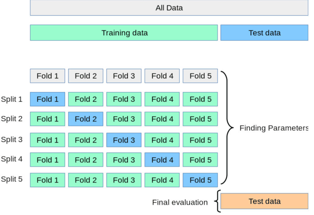
This method begins by randomly separating the data into k subsets, one of which is used as a validation data set and the other k-1 are used for training on. After that one of the subsets that was just used as a training subset is now used as a validation subset, and the old validation subset is now used for training. This process repeats until every one of the k subsets has been used as the validation set exactly once. The results are then averaged over all repeats. Here’s a graphic to illustrate the method.
Sourced from the scikit-learn docs here
This graphic is using a 5-fold cross-validation. You can see how each subset gets exactly one chance at being the validation set. For every row (named ‘split’ on the figure) the model is trained on the green data and tested on the blue data.
A further advancement on the method is called stratified k-fold cross-validation. This is the same approach except each subset in the partition (each ‘fold’) is chosen to preserve the distribution of classes present in the whole training set. This is in fact the method we will use later on, however we will not be coding it by hand (yet).
The value for k that we choose can depend on a number of factors but I am currently unsure on the best practices and reasons for picking a certain k. As such I am going to arbitrarily choose k = 10 for my dataset. You could even pick multiple values for k and then run all the tests again on each new value.
Testing Algorithms
Ideally we want to test between 10-20 different algorithms of varying types. For example, we want some of the algorithms to be regression, some to be instance-based, some could be neural networks, etc. At the start of the project I was unsure if there were particular algorithms I should be targeting for this particular dataset. I chose a random list but some algorithms were completely unsuitable. Here is the list of algorithms I have ended up trialling after various previous failures:
- Logistic Regression
- k-Nearest Neighbour
- Support Vector Machines
- Ridge Regression
- Classification and Regression Tree
- Gaussian Naive Bayes
- Multinomial Naive Bayes
- Multilayer Perceptrons
- Linear Discriminant Analysis
- Quadratic Discriminant Analysis
Note: some of the original algorithms on the list were Linear Regression and Elastic Net. I tried them on the problem and they threw loads of errors and eventually I discovered these algorithms are not suitable for a classification problem. But now I know! You have to make these mistakes to learn so don’t be afraid to throw any algorithm at a problem to see what sticks.
This list is full of intimidating names but don’t worry if you have no idea what any of them mean – I barely know myself! We’re not going to be coding any of them ourselves or even understanding how they work. We will just apply standard implementations of them for now and work on the results they give. In the future I expect to be covering how we can code them by hand but for now that isn’t our concern.
So we’ve planned our approach. Let’s get to some coding!
Writing The Code
So maybe this is your first time writing any code for a machine learning project. It’s quite intimidating especially with all the garble I’ve written above but I’ll go slowly. If you want to follow along, feel free to download the Iris flower dataset from the UCI Machine Learning Repository. Also my code files are uploaded to GitHub here.
Visualising The Dataset
The best thing to do when we download a new dataset is to just have a look at it! Let’s print out the first few lines and plot some of the data. Note that for loading the dataset I’m using the ‘pandas’ library, so make sure to import that first.
We can load up the dataset as follows. Either a file path or a URL can be used for loading the data.
We will use some incredibly important functions to have a quick peek at the data. These are the kind of functions I’ll be using on every dataset I ever load. Here are four of them:
dataset.shape will give us the dimensions of the set. Here it prints:

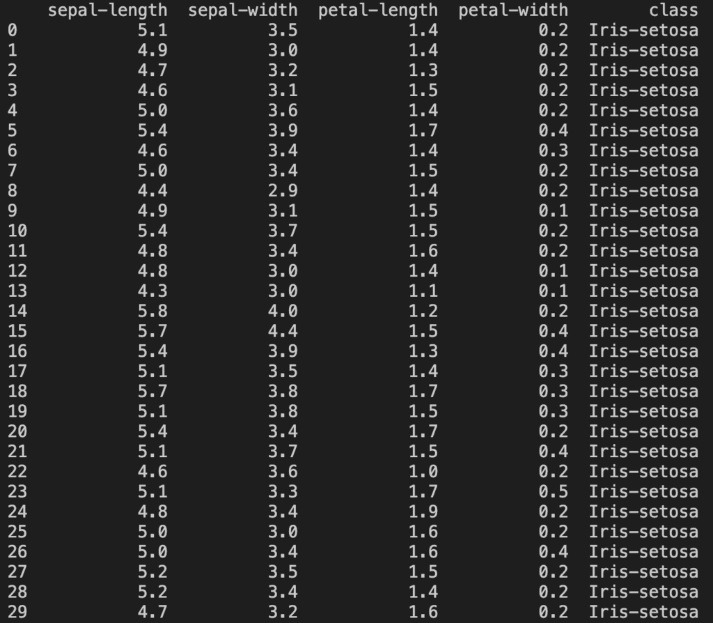
dataset.head(n) will print out the first n lines of the set. Here it prints:
dataset.describe() gives us the count, mean, std, min, Q1, Q2, Q3, and max value of every attribute in the dataset. Here it prints:

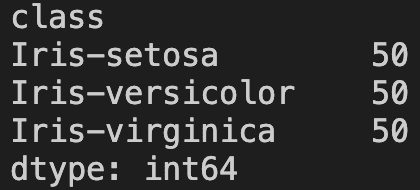
dataset.groupby(‘class’).size() tells us how many of each class is in the dataset. Here it prints:
Plotting the Data
That immediately gives us a great overview of the data! But we can go further. Let’s plot some graphs. Here is the code to create a box plot, histogram and scatter matrix (aka. pairplot) for the data.
This code will give the following three plots.
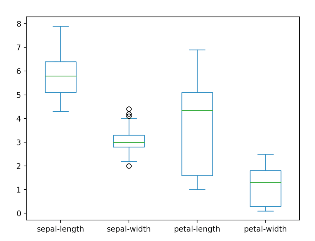
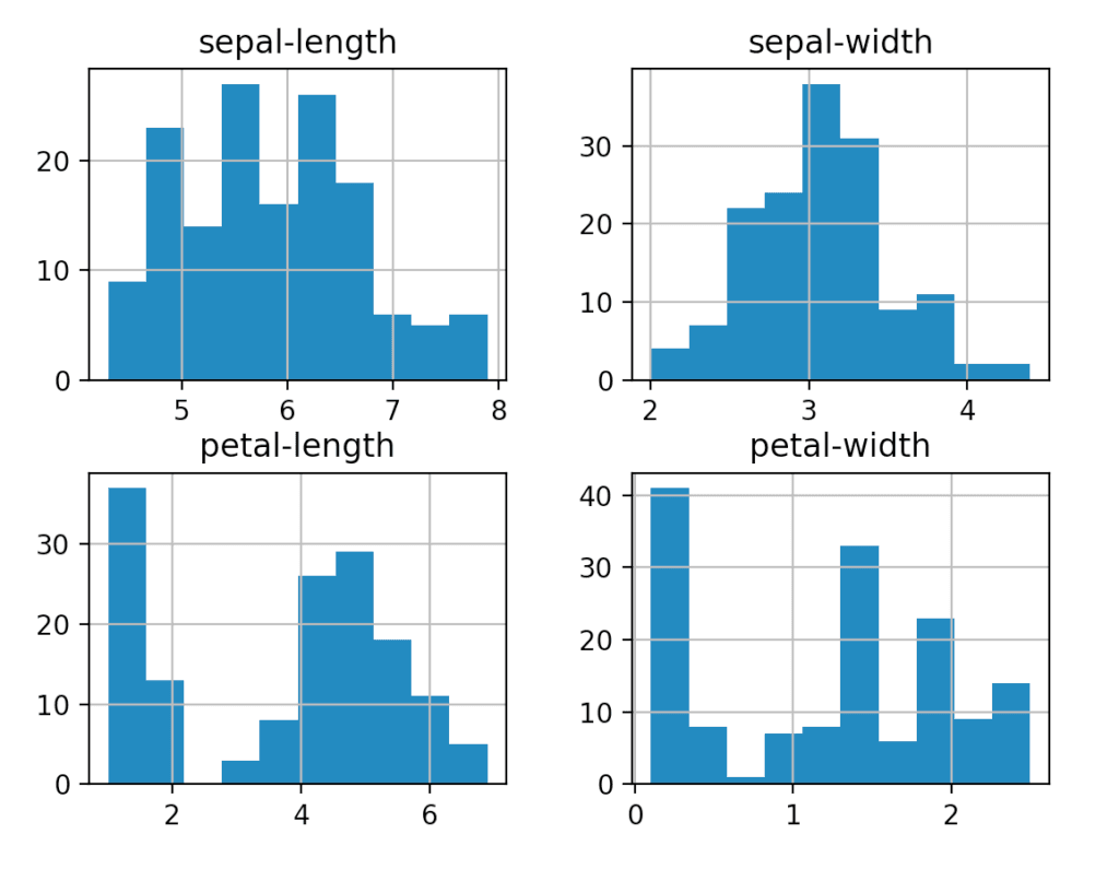
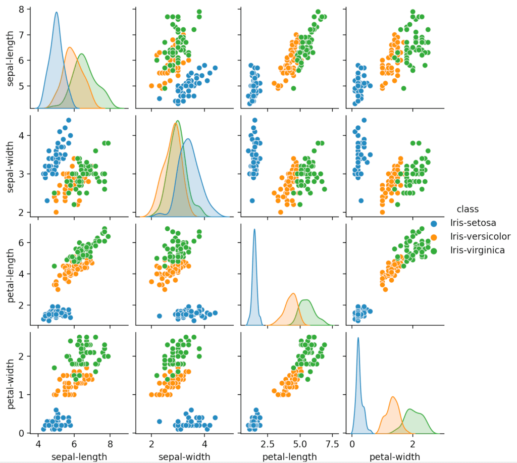
The box plot is useful for comparing multiple groups of data. It gives a high-level, glanceable summary of some key features we might be interested in.
A histogram is more in-depth than the box plot and allows us to see the distribution of the data. This can help us make some inferences about the kind of model we might want to use. For example, the ‘sepal-width’ seems to resemble a Gaussian distribution which we may be able to exploit when searching for a model. We can also change the number of bins the histogram uses (by adding a ‘bins = n’ argument) which can help to reveal distributions.
The scatter matrix / pairplot allows us to see the relations between all different pairs of attributes. We can use it to see correlations between these pairs. For example, petal width and petal length seem to be quite strongly positively correlated.
Partitioning The Data
First we need to partition our data into two. We need a training set to train the model and a validation set to test the model. I will opt to take a 20% split of the data for validation, but you could choose 25%, 33%, etc.
Converting the Dataset into Two Python Lists
To create a train/test split we first need to turn our dataset into a python list which can be done via accessing the ‘values’ property of the dataset.
Here are the first ten lines of the output:
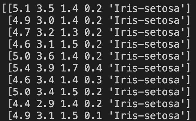
Now we need a new list to hold the first four attributes and another new list to hold the corresponding classes. This can be done in the following way:
To confirm we’ve done it correctly it’s always best to print out the new X and y. Here are the first ten lines of X and then y:
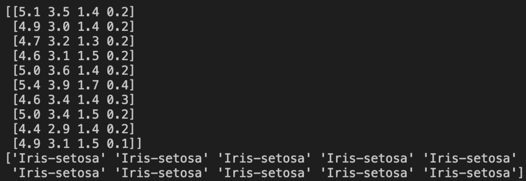
Creating the Train/Test Split
We can now pass X and y into one of the sklearn functions called ‘train_test_split’ to partition the dataset into an 80/20 split.
Note that the ‘random_state = 1’ basically applies a consistent seed to the shuffling that is done to the data before it is sampled into partitions. Providing a shuffling seed means that we get the same partitions every time we run the code. To get an idea of what ‘train_test_split’ has returned we can simply print the length of the four lists:
Outputs:

So indeed we now have 20% of the data separated into two validation lists. One list holds the four attributes, the other holds the classes associated to the attributes. Importantly, the nth element of ‘X_train’, say, is associated to the nth element of ‘Y_train’, as it was in the original list; we have not lost the connection between the measurements of the flowers and the class of flower these measurements belong to.
We now have our data partitioned and ready to be used!
Finding A Model
This is where we want to start applying off-the-shelf algorithms to our data to get a general idea of what works and what doesn’t. Let’s initialise all the models and add them to a list:
Implementing K-Fold Cross-Validation
This is where we finally need to implement the 10-fold cross-validation that I talked about earlier. We will use the ‘StratifiedKFold’ object in sklearn. Here is how we can initialise the object and then return our folds:
This gives us two arrays of indices per fold: one for training and one for testing. Note that earlier we already split the data into a training set and a validation set so it’s easy to get confused here. We are further breaking up the original training set (but we do NOT touch the original validation set) into 10 different partitions that each contain their own training set and validation set. Refer to Figure 1 above for a graphical explanation of this.
Here are the first four folds output by the above code (of course it continues to ‘Fold 9’ but you get the idea from the first four):
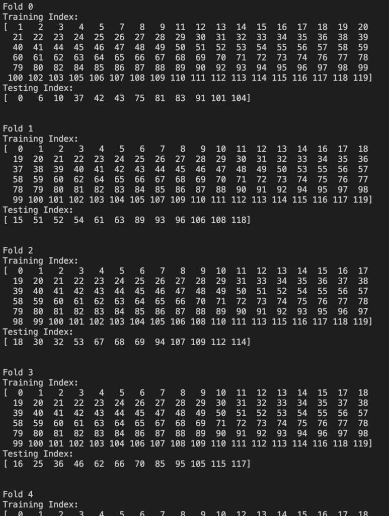
So now we can access our datasets at each of these indices to train and test each model over all the ten folds.
I thought it would be useful to spell out how the ‘StratifiedKFold’ object works because the next function we use (‘cross_val_score’) does all of this behind the scenes and it’s not particularly intuitive. Let’s have a look at that now.
Performing Cross-Validation on the Models
We want to loop through the list of models we made earlier and apply each of them to the training set. We’ll apply every model to all ten folds then give each one an average accuracy score.
So the highlight here is the ‘cross_val_score’ function. We provide it with the ‘StratifiedKFold’ object and it goes ahead and creates the index arrays for the folds (like we did earlier), runs the current model on all these ten folds and then returns the accuracy score (accuracy is correct predictions divided by all predictions).
Upon running this loop all the models worked fine except for Logistic Regression which wasn’t able to converge. I can think of two ways to solve this: rescale the data or change some model parameters. I changed the ‘solver’ parameter to ‘liblinear’ which fixed the convergence issue (I don’t necessarily know why it fixed it however). So here is all the code so far.
The results we get are:
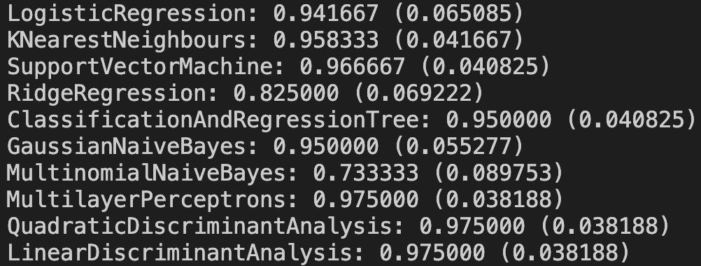
The first number is the mean classification accuracy and the second is standard deviation.
Picking a Model
Ideally at this point we would perform a hypothesis test on the models to determine if the difference in performance of one model was statistically significant when compared to the others. However I don’t want to tackle too much for our first project so I’m going to simply choose the model that appears to have the best accuracy. It seems that Multinomial Naive Bayes model has the worst performance on the data while the three last models are the best. Again if I was really trying to find the best model I would then dive into different models that are similar to Multilayer Perceptrons and Linear/Quadratic Discriminant Analysis to try to find an even better performer. We’ll simply settle for choosing the Linear Discriminant Analysis model because it runs the fastest and is the simplest of the highest scorers.
Testing the Model
So we’ve picked Linear Discriminant Analysis as a well performing model over our training data. Let’s now focus on this model individually and run it on the validation set that we originally separated.
The results we obtain are:
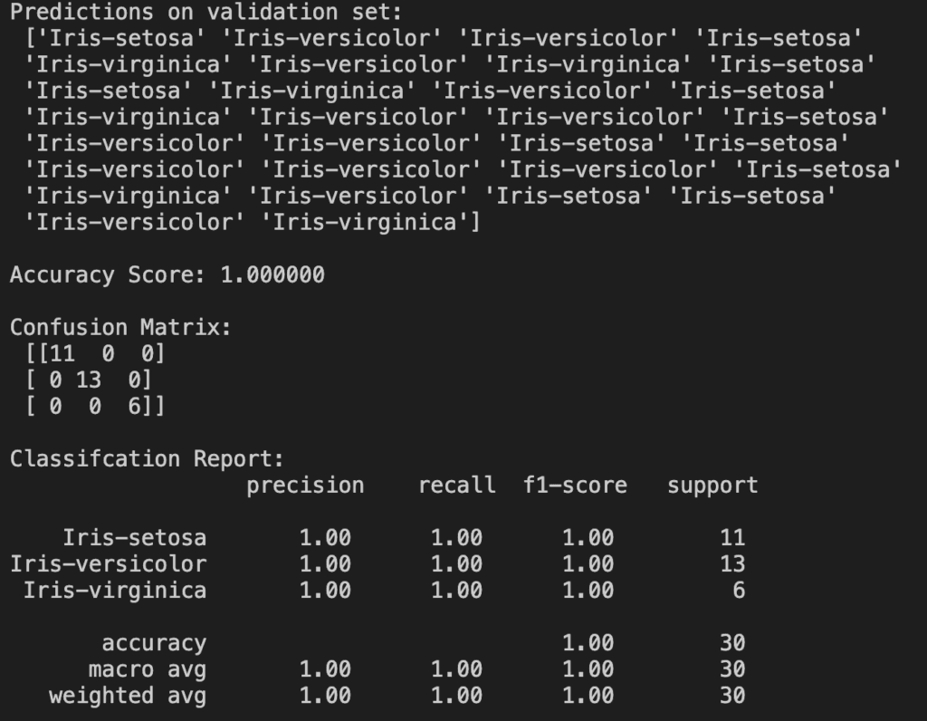
The first thing we notice is an accuracy score of 100%! That is obviously very good (perfect, in fact) but remember this validation set contains only 30 rows of data. Doesn’t stop me being happy though!
The confusion matrix tells us where the model made errors. Numbers on the diagonal are correct guesses but numbers anywhere else are errors. Since we were 100% accurate all numbers are on the diagonal.
The classification report gives us some additional performance metrics for each class. We don’t need to know what all these mean for now. In any case it’s not too useful to us since they are all 1!
I’ve also printed out all the model’s raw predictions at the top because I think it’s cool to see our program actually making its own guesses on new data. Without printing this we might lose sight of what the model’s actual purpose is.
Improving Results
If we were doing an in-depth project for real we would want to fine-tune the model we found. I am not going to do this because we’ve covered a lot of ground already and this is my first project! I don’t want to cover too much too fast. We can however discuss how we might pursue that objective.
I would first try to make a top three list of the best performing models from our spot-check, using statistical significance tests to ensure we are making justified decisions. Then I would pick other algorithms that we didn’t try that are similar to those in the top three. Again we could pick the top three performers from these new algorithms.
At this point we should be trying to fine-tune each of these three best algorithms by fiddling with their parameters. We could do some sort of sensitivity analysis to do this. We will likely have pretty good models after doing that but we can go further and perhaps use some standard ensemble methods to combine the best performers into one model. This is useful if our best models specialise or perform better than average on particular things – we can combine their specialisations together.
The final thing we might try is feature engineering. This is when we modify the structure of the dataset by combining/separating attributes into new forms. Some models might work better on differently structured data so we might as well try to find if there is some optimal form for the dataset. Note that each time we change the dataset, we should repeat the entire model selection process again to give everything a fair chance.
Presenting Our Results
This is an important part of our project and should not be ignored. We want to write up what we learnt so that we can reference the results for future projects.
Let’s refer to the first section where we defined the problem. I wanted “a program which can tell me what type of flower I have, from measurements of its sepals and petals”. That is exactly what I’ve produced in the final code snippet above. Well done me!
Learning Points
I said that the solution would be used to learn about some strengths and weaknesses of machine learning algorithms on classification tasks. So here’s what I learnt over the course of the project:
- Clustering methods are intended for use on unsupervised data so are not the most appropriate to this problem. I originally had k-means included on my algorithms list but it gave an accuracy of 0 so I removed it as it was not appropriate to the problem.
- Generally regression algorithms are not for classification, they are intended for guessing real number values. I tried to use Linear Regression and Elastic Net on this data but it threw a lot of errors forcing me to look into why they wouldn’t work. They were expecting floats in place of where I had the strings representing the classes.
- I learnt a lot about setting up tests for algorithms, ie. using k-fold cross-validation. As for picking the k value, I simply defaulted to 10 which I think is a safe choice. Perhaps repeating tests for all algorithms with different k values would be a good idea in the future.
- I found out about the importance of data visualisation at the start of the project. You need to know what your data looks like so that you know exactly what you’re working with. It can also help to guess the data’s distribution. I now know how to plot box plots, histograms and scatter matrices for datasets.
- I am more familiar with the process of finding a machine learning model. I know to choose multiple algorithms of different types and use a cross-validation approach to assess their performance. I know of some of the additional methods to apply after this too.
Model Performance
The model we ended up picking did perform very well on the validation data, scoring 100% accuracy. Ideally I would like some more data to test it on because it’s hard to see the limitations of the model when it doesn’t have enough test data. It also means we cannot easily tune the model because it already achieves the maximum accuracy score.
Conclusion
This is our first project completed! I hope you’ve learned a lot about applied machine learning from this. I definitely have as I needed to do a lot of research to work the project through to the end. In the future I may return to this dataset and try the extension tasks I detailed, including feature engineering or ensemble methods for combining our best models. However for the projects that immediately follow this one, I think it would be wise to try and use the techniques I learnt but on a bigger, more difficult dataset.
I’ll leave the code for download on GitHub if you’re interested in viewing it in full. Follow this link for that.
See you for the next project!