Coding a Naive Bayes Classifier in Python

The Naive Bayes Classifier is very simple, effective and one of the most efficient classifiers available. It's often a good test model to throw at a problem due to it's speed and ability to train effectively from a small sample of data.

It utilises Bayes Theorem together with some naive independence assumptions between the attributes and, even though this assumption almost never holds, it performs surprisingly well on complex problems. Feel free to follow this link for a deep dive on why Naive Bayes works well, despite not satisfying it's assumption.

Today our goal will be to code a Gaussian Naive Bayes classifier from scratch in Python! We'll start by taking a brief look at the mathematical theory, then we will look at how the theory can be turned into an implementation, and finally we will carry out this implementation and test it on a simple dataset.

Naive Bayes Classifier coded from scratch in Python Photo by Frank_am_Main, some rights reserved.

Theory

The Naive Bayes learning algorithms are derived through the use of Bayes Theorem together with conditional independence assumptions. We'll talk about the condition soon but for now independent just means that all the attributes (columns of the dataset) do not influence each other at all.

Let's take a look at Bayes Theorem. It states that for events $A$ and $B$ :

P(A|B) = \dfrac{P(B|A)P(A)}{P(B)}, \text{where } P(B) \not= 0

Our goal is to determine the probability that, when given some data, it belongs to one of the possible classes. We can see that by setting A = class, B = data, Bayes Theorem becomes applicable to our problem. P(class|data) is the probability that the data belongs to the class. Perfect!

However a piece of data in a dataset will be represented by a feature vector - a vector where the ith element corresponds to the value in the ith column of the dataset. So we could say:

data = (x_1, x_2, \cdots, x_n)

So given a particular $data$ , the probability that it belongs to the class $c$ is:

P(c|x_1, x_2, \cdots, x_n) = \dfrac{P(x_1, x_2, \cdots, x_n|c)P(c)}{P(x_1, x_2, \cdots, x_n)}

The naive conditional independence assumption states that, given a class $c$ , all of the features in the data (each of the $x_i$ ) are independent. That is to say:

$P(x_1, x_2, \cdots, x_n|c) = \prod\limits_{(i = 1)}^{n}P(x_i|c)$

So we can substitute this into the previous equation to obtain:

P(c|x_1, x_2, \cdots, x_n) = \dfrac{P(c)\prod_{i=1}^{n}P(x_i|c)}{P(x_1, x_2, \cdots, x_n)}

But then given some fixed $(x_1, x_2, \cdots, x_n)$ , the quantity given by $P(x_1, x_2, \cdots, x_n)$ is constant too, so we can further simplify:

P(c|x_1, x_2, \cdots, x_n) \varpropto P(c)\prod\limits_{(i = 1)}^{n} P(x_i|c)

Now given a feature vector, this formula can calculate the probability that it belongs in each class... well not exactly. When we simplified by removing the denominator, we suddenly stopped representing the actual probability value. However for our purposes, all we need is the proportionality. So we compute all the relevant quantities and then compare them to find the largest. As such, the natural classification rule would be to assign the feature vector (data) to the class with the highest calculated value. If we denote the predicted class as $\hat{c}$ , then this rule can be written down as:

\hat{c} = \underset{c}{\mathrm{argmax}}P(c)\prod\limits_{i=1}^{n}P(x_i|c)

This is the formula we need to develop an algorithm. If we can figure out how to calculate the right hand side, then we have the predicted class for a data point.

Developing The Algorithm

Our sole task for the algorithm is to figure out how to enumerate:

\underset{c}{\mathrm{argmax}}P(c)\prod\limits_{i=1}^{n}P(x_i|c)

$P(c)$ is the probability of the class $c$ . We can calculate this by counting how many samples in our dataset belong to class $c$ , and then dividing this by the total number of samples in the dataset.

To evaluate each term in the product we need to understand how to calculate the probability of observing the given value $x_i$ . This is where the various Naive Bayes models differ because we have to make an assumption on what the distribution of $P(x_i|c)$ is. In our case, we will assume a Gaussian distribution (which gives rise to the Gaussian Naive Bayes model), but other applications may use a Multinomial or Bernoulli distribution, for example. The Gaussian distribution is also known as the Normal distribution or, informally, 'bell curve'.

So to determine $P(x_i|c)$ we need to understand how to use the Gaussian probability density function. This is how we find the probability of observing the given real number. So the probability of observing $x$ is:

f(x) = \dfrac{1}{\sigma \sqrt{2\pi}}e^{-\dfrac{1}{2}\left(\dfrac{x-\mu}{\sigma}\right)^{2}}

However you may be wondering how we make this number conditional on the class $c$ , as we require. That problem is easily solvable by using the above equation, but substituting different values of $\sigma$ (the standard deviation of the class) and $\mu$ (the mean of the class), corresponding to which class we are considering.

So if we had three different classes A, B, and C, each with four columns, and we were trying to classify the data point $x$ , we would need to individually calculate the mean and standard deviation for each column in A, then in B, then in C, and store all these twenty-six values separately (3 classes _ 4 columns in each class _ 2 values to calculate for each column = 26). Then we could correctly plug these parameters into the formula above and find the probability of observing $x$ , conditionally on each class.

Let's quickly remind ourselves how to calculate the mean and standard deviation:

For a set of values $x_i$ , the mean is given by:

\mu = \dfrac{\sum_{i=1}^{N}x_i}{N}

The mean is then used to calculate the Bessel corrected standard deviation, which is given by:

\sigma = \sqrt{\dfrac{1}{N-1}\sum\limits_{i=1}^{N}(x_i-\mu)^{2}}

Let's combine everything we've talked about into a numbered list:

Group all samples in the dataset by class 2. Within each class, for each feature (column), calculate the mean, standard deviation, and sample count (this number is needed to calculate the proportion of samples in each class, P(c)), from the samples present. Calculating these parameters encompasses the training process for the model.
For new data, use the mean and standard deviation corresponding to each feature within each class in turn to calculate the conditional probability that this data belongs to each class (this uses the formula above). We'll then need to compare these probabilities between all classes and choose the class with the highest probability associated with it. This will be our model's final prediction. 4. Not part of the algorithm, but we should implement a model evaluation function to ensure we've implemented the algorithm correctly.

This whole list encompasses the algorithm we will be coding!

Are We Using Libraries?

Short answer: yes, but only pandas and sklearn.model_selection.train_test_split

This is an important question because it affects the scope of where the challenge lies in this project. My goal that I've chosen is to code a Gaussian Naive Bayes classifier by hand. For this reason I don't want to also focus on coding train/test splits, CSV readers, or data manipulation algorithms by hand. These problems could be separate projects. As such, I will import pandas and scikit-learn's train_test_split function, but if you want to do the whole project without libraries that is very possible, but I leave that as a challenge for you!

Loading The Test Dataset

If we’re coding a classifier then we need some data to test it! As I just mentioned, the focus of the project is coding a classifier by hand so we don’t want to focus much on the data or have to do any real processing with it. As such the best choice is to use the Iris Flower Dataset because it is very small and very simple. Let’s load it up and take a peek at the data.

python

import pandas as pd

dataFilepath = 'YOUR FILEPATH/iris.data'
columns = ['sepal-length', 'sepal-width', 'petal-length', 'petal-width', 'class']
dataset = pd.read_csv(dataFilepath, names=columns)

print(dataset.head())

This gives us the first five lines of data:

plaintext

sepal-length  sepal-width  petal-length  petal-width        class
0           5.1          3.5           1.4          0.2  Iris-setosa
1           4.9          3.0           1.4          0.2  Iris-setosa
2           4.7          3.2           1.3          0.2  Iris-setosa
3           4.6          3.1           1.5          0.2  Iris-setosa
4           5.0          3.6           1.4          0.2  Iris-setosa

Now we know the basic structure of the set. We have four numerical attributes along with the ‘class’ column.

Let’s check the number of data points we have, and also how the classes are distributed.

python

...
print(dataset.shape)
print(dataset['class'].value_counts())

This outputs:

plaintext

(150, 5)
Iris-setosa        50
Iris-versicolor    50
Iris-virginica     50

So we have 150 data points in the full set, and the classes are completely balanced; each class contains 50 members.

Great! Now we have some data and can start producing the algorithm!

Implementing The Algorithm

In order to start developing and testing our algorithm, I’m going to first trim down the dataset into a ‘toy’ size, consisting of just the first five elements from each class. This lets us see an entire (toy) dataset at once and allows us to better understand what our code is doing.

python

...
smallDataset = pd.concat([dataset[0:5], dataset[50:55], dataset[100:105]]).reset_index(drop=True)
print(smallDataset)

This shows our full new ‘toy’ set:

plaintext

sepal-length  sepal-width  petal-length  petal-width            class
0            5.1          3.5           1.4          0.2      Iris-setosa
1            4.9          3.0           1.4          0.2      Iris-setosa
2            4.7          3.2           1.3          0.2      Iris-setosa
3            4.6          3.1           1.5          0.2      Iris-setosa
4            5.0          3.6           1.4          0.2      Iris-setosa
5            7.0          3.2           4.7          1.4  Iris-versicolor
6            6.4          3.2           4.5          1.5  Iris-versicolor
7            6.9          3.1           4.9          1.5  Iris-versicolor
8            5.5          2.3           4.0          1.3  Iris-versicolor
9            6.5          2.8           4.6          1.5  Iris-versicolor
10           6.3          3.3           6.0          2.5   Iris-virginica
11           5.8          2.7           5.1          1.9   Iris-virginica
12           7.1          3.0           5.9          2.1   Iris-virginica
13           6.3          2.9           5.6          1.8   Iris-virginica
14           6.5          3.0           5.8          2.2   Iris-virginica

Let’s use this to start going through our numbered list.

1. Group Samples By Class

To group samples by the ‘class’ column, I will be using the pandas ‘groupby()’ function. This will initially give us a dictionary of indices:

python

...
dataByClass = smallDataset.groupby('class').groups
print(dataByClass)

Outputs:

plaintext

{'Iris-setosa': [0, 1, 2, 3, 4], 
'Iris-versicolor': [5, 6, 7, 8, 9], 
'Iris-virginica': [10, 11, 12, 13, 14]}

So we will now need to access the actual value stored at these indices. Let’s combine all this into a function:

python

def SeparateClasses(dataset):
  # Function separates the classes in a dataset, saving the result as a dictionary with classes as the keys.
  separateClassesDict = {}
  dataByClass = dataset.groupby('class')

  for group, data in dataByClass:
      separateClassesDict[group] = data
   
  return separateClassesDict

...

dataByClass = SeparateClasses(smallDataset)

for x in dataByClass.keys():
  print(x)
  print(dataByClass[x])

This now outputs:

plaintext

Iris-setosa
 sepal-length  sepal-width  petal-length  petal-width        class
0           5.1          3.5           1.4          0.2  Iris-setosa
1           4.9          3.0           1.4          0.2  Iris-setosa
2           4.7          3.2           1.3          0.2  Iris-setosa
3           4.6          3.1           1.5          0.2  Iris-setosa
4           5.0          3.6           1.4          0.2  Iris-setosa
Iris-versicolor
 sepal-length  sepal-width  petal-length  petal-width            class
5           7.0          3.2           4.7          1.4  Iris-versicolor
6           6.4          3.2           4.5          1.5  Iris-versicolor
7           6.9          3.1           4.9          1.5  Iris-versicolor
8           5.5          2.3           4.0          1.3  Iris-versicolor
9           6.5          2.8           4.6          1.5  Iris-versicolor
Iris-virginica
  sepal-length  sepal-width  petal-length  petal-width           class
10           6.3          3.3           6.0          2.5  Iris-virginica
11           5.8          2.7           5.1          1.9  Iris-virginica
12           7.1          3.0           5.9          2.1  Iris-virginica
13           6.3          2.9           5.6          1.8  Iris-virginica
14           6.5          3.0           5.8          2.2  Iris-virginica

You can see how each class now holds its samples in separate datasets. This is exactly what we wanted to achieve so let’s move to the next objective!

2. Calculating Mean and Standard Deviation For Columns

The natural place to start would be coding functions to calculate mean and standard deviation. Refer to the equations above if you need a refresher on the formulas. Here are the two functions:

python

def Mean(data):
  return sum(data)/len(data)

def Std(data):
  mu = Mean(data)
  newList = [(x-mu)**2 for x in data]
  return math.sqrt((1/(len(data)-1))*sum(newList))

These follow precisely from the formulas so hopefully the implementation makes sense. For clarity, I’ve separated out a variable to hold the list comprehension in the ‘Std’ function. This list just holds the squared, mean-corrected values of the input data. For robustness, I should do checks for things like empty lists, but since this is just a personal project I’m not worrying about covering all cases. You can try coding this check yourself!

Let’s test them to make sure they work as intended:

python

print('Mean: ' + str(Mean([1,2,3,4,5,6,7,8])))
print('Std: ' + str(Std([1,2,3,4,5,6,7,8])))

This outputs:

plaintext

Mean: 4.5
Std: 2.449489742783178

If we calculate these statistics by hand we see the same numbers, hence our implementation seems correct.

Now we want to call these functions to calculate the mean and standard deviation for each column of each class. Moreover, we want to keep a count of how many samples are contained in each class so that we can calculate the class probability. Below is a more graphical explanation. Note that I just show the ‘Iris-setosa’ class at the top but the same happens to all three classes:

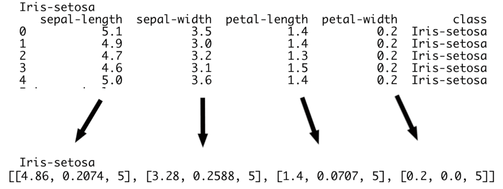
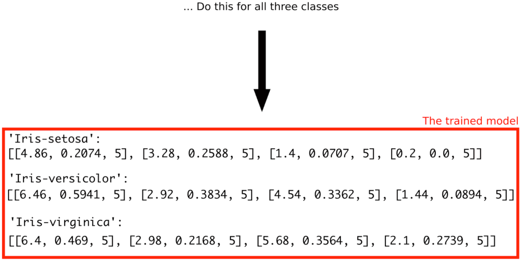
Printout of the first 4 rows of the dataset with arrows linking each column to a list of its mean, standard deviation and sample count

Printout of lists of mean, standard deviation and sample count for each of the columns of each of the three different classes in the set

The lists here are [mean, standard deviation, number of samples].

The red box here shows what our trained model will look like. It is a dictionary where each key represents a class and holds four lists (corresponding to four attributes), each containing the mean, standard deviation and sample count of a different column in that class.

So our first job is to write a function that takes in a single class and calculates, for each column, the mean, standard deviation and sample count. The following code handles this task:

python

def CalculateColumnStatsForGivenClass(singleClassDataset):
  # Function calculates the mean, std and sample count for each column, given a single class
  requiredList = []

  # Get all the column names in this class as a list
  cols = list(singleClassDataset.columns)

  # Loop through the list of column names, calculating mean, std, and sample count
  for x in list(cols[0:len(cols)-1]): # -1 because we don't want to include the column for 'class'
      requiredList.append([Mean(singleClassDataset[x]), Std(singleClassDataset[x]), len(singleClassDataset[x])])
  return requiredList

Here I am simply looping through all the columns in the given set and, for each one, appending a list of the stats we want to ‘requiredList’.

Let’s test this out on the ‘Iris-versicolor’ class:

python

...
dataByClass = SeparateClasses(smallDataset)
classStats = CalculateColumnStatsForGivenClass(dataByClass['Iris-versicolor'])
print(classStats)

This outputs:

plaintext

[[6.459999999999999, 0.594138031100518, 5], 
[2.9200000000000004, 0.38340579025361643, 5], 
[4.540000000000001, 0.3361547262794323, 5], 
[1.44, 0.08944271909999157, 5]]

This seems good! Recall that the first sub-list here corresponds to the mean, standard deviation and sample count of the first attribute (column) of ‘Iris-versicolor’ (which is ‘sepal-length’), and the second sub-list is these stats for the second attribute (which is ‘sepal-width’), and so on for all four attributes.

Now we need to call this function on every class and save each list produced in a dictionary. This will produce the full model. Let’s write another function to do that:

python

def TrainModel(dataset):
  # Function produces a dictionary representing the Gaussian naive bayes model. 
  result = {}

  # First separate the classes
  dataSeparatedByClassDict = SeparateClasses(dataset)

  # Loop through each class
  for x in list(dataSeparatedByClassDict.keys()):
      # Calculate the mean and std for each attribute, within each class
      result[x] = CalculateColumnStatsForGivenClass(dataSeparatedByClassDict[x])
  return result

This code will loop through all the keys in the dictionary (ie. all the classes in the dataset) and then produce a new dictionary with the same keys, but now the keys correspond to the lists of [mean, standard deviation, sample count], rather than just the raw data.

So lets call this on our small dataset:

python

...
model = TrainModel(smallDataset)
for x in model.keys():
  print(x)
  print(model[x])

This outputs:

plaintext

Iris-setosa
[[4.859999999999999, 0.2073644135332772, 5], [3.28, 0.2588435821108957, 5], [1.4, 0.07071067811865474, 5], [0.2, 0.0, 5]]
Iris-versicolor
[[6.459999999999999, 0.594138031100518, 5], [2.9200000000000004, 0.38340579025361643, 5], [4.540000000000001, 0.3361547262794323, 5], [1.44, 0.08944271909999157, 5]]
Iris-virginica
[[6.4, 0.4690415759823429, 5], [2.98, 0.21679483388678789, 5], [5.680000000000001, 0.35637059362410944, 5], [2.1, 0.2738612787525831, 5]]

I’ll put the full ‘smallDataset’ here as well so you can compare where these numbers have come from.

plaintext

sepal-length  sepal-width  petal-length  petal-width            class
0            5.1          3.5           1.4          0.2      Iris-setosa
1            4.9          3.0           1.4          0.2      Iris-setosa
2            4.7          3.2           1.3          0.2      Iris-setosa
3            4.6          3.1           1.5          0.2      Iris-setosa
4            5.0          3.6           1.4          0.2      Iris-setosa
5            7.0          3.2           4.7          1.4  Iris-versicolor
6            6.4          3.2           4.5          1.5  Iris-versicolor
7            6.9          3.1           4.9          1.5  Iris-versicolor
8            5.5          2.3           4.0          1.3  Iris-versicolor
9            6.5          2.8           4.6          1.5  Iris-versicolor
10           6.3          3.3           6.0          2.5   Iris-virginica
11           5.8          2.7           5.1          1.9   Iris-virginica
12           7.1          3.0           5.9          2.1   Iris-virginica
13           6.3          2.9           5.6          1.8   Iris-virginica
14           6.5          3.0           5.8          2.2   Iris-virginica

This brings us to the end of the second objective. We can now train the parameters of our Naive Bayes model! Here is the full code so far:

python

import pandas as pd
import math

def SeparateClasses(dataset):
  # Function separates the classes in a dataset, saving the result as a dictionary with classes as the keys.
  separateClassesDict = {}
  dataByClass = dataset.groupby('class')

  for group, data in dataByClass:
      separateClassesDict[group] = data
   
  return separateClassesDict

def Mean(data):
  return sum(data)/len(data)

def Std(data):
  mu = Mean(data)
  newList = [(x-mu)**2 for x in data]
  return math.sqrt((1/(len(data)-1))*sum(newList))

def CalculateColumnStatsForGivenClass(singleClassDataset):
  # Function calculates the mean, std and sample count for each column, given a single class
  requiredList = []

  # Get all the column names in this class as a list
  cols = list(singleClassDataset.columns)

  # Loop through the list of column names, calculating mean, std, and sample count
  for x in list(cols[0:len(cols)-1]): # -1 because we don't want to include the column for 'class'
      requiredList.append([Mean(singleClassDataset[x]), Std(singleClassDataset[x]), len(singleClassDataset[x])])
  return requiredList

def TrainModel(dataset):
  # Function produces a dictionary representing the Gaussian naive bayes model. 
  result = {}

  # First separate the classes
  dataSeparatedByClassDict = SeparateClasses(dataset)

  # Loop through each class
  for x in list(dataSeparatedByClassDict.keys()):
      # Calculate the mean and std for each attribute, within each class
      result[x] = CalculateColumnStatsForGivenClass(dataSeparatedByClassDict[x])
  return result

if __name__ == '__main__':
  # Load the dataset
  dataFilepath = 'YOUR FILEPATH/iris.data'
  columns = ['sepal-length', 'sepal-width', 'petal-length', 'petal-width', 'class']
  dataset = pd.read_csv(dataFilepath, names=columns)

  # Create toy dataset
  smallDataset = pd.concat([dataset[0:5], dataset[50:55], dataset[100:105]]).reset_index(drop=True)

  # Train the model on the dataset
  model = TrainModel(smallDataset)
  for x in model.keys():
      print(x)
      print(model[x])

3. Calculating Classification Probability for New Data

To calculate the probability that new data belongs to each class we need to finally invoke the theory we looked at previously. In particular, we are interested in calculating:

\underset{c}{\mathrm{argmax}}P(c)\prod\limits_{i=1}^{n}P(x_i|c)

The first term, $P(c)$ , is the probability of observing a class which we can calculate as the proportion of each class in the set. So for our case we know this value is about 33% for all classes since they are balanced. However we will code it to deal with the general case and assume we don't know this. Here is a function that achieves this:

python

def CalculateProbabilityOfClassC(c, model):
  # Function computes the probability of a class c, using counts of how many samples are in each class.
  numberOfSamplesInClassC = model[c][0][2]
  numberOfSamplesInTotal = sum([model[x][0][2] for x in list(model.keys())])
  return numberOfSamplesInClassC/numberOfSamplesInTotal

There are multiple layers of indexing here which is not too intuitive so let me break it down. Recall that a given key in the dictionary called ‘model’ contains a list that looks like this:

plaintext

[[6.459999999999999, 0.594138031100518, 5],
[2.9200000000000004, 0.38340579025361643, 5],
[4.540000000000001, 0.3361547262794323, 5],
[1.44, 0.08944271909999157, 5]]

So this example list would correspond to model[c] in the function. Then, since we are interested in how many samples of this class exist, we want to access the 3rd element of each sub-list (ie. 5). But all of these 3rd elements are the same so I just take the first sub-list. So extracting the number 5 here corresponds to model[c][0][2].

Then we do this same process within a list comprehension so that we can add up how many samples there are over all classes in the whole dataset. For our small dataset, I will print what that list looks like:

plaintext

[5, 5, 5]

So summing the elements of this list tells us how many samples are in the whole set.

Finally we just divide these numbers to find the proportion of samples belonging to class c in the whole set.

Let’s test an example:

python

...
model = TrainModel(smallDataset)
print(CalculateProbabilityOfClassC('Iris-setosa', model))

Outputs:

plaintext

0.3333333333333333

As expected!

Now we need to cover the second term which is the scary-looking product. Fortunately this is relatively straightforward! Since we are implementing a Gaussian Naive Bayes model, we will calculate this using a Gaussian PDF. The calculation will require implementing the following formula:

P(x_i|c) = \dfrac{1}{\sigma_{c_i} \sqrt{2\pi}}e^{-\dfrac{1}{2}\left(\dfrac{x_i-\mu_{c_i}}{\sigma_{c_i}}\right)^{2}}

Where $x$ is a new row of data, and $x_i$ is the value in the ith attribute (column) of that data, $c$ is a given class, $\mu_{c_i}$ is the mean of the values in the ith attribute of class $c$ , and $\sigma_{c_i}$ is the standard deviation of the values in the ith attribute of class $c$ .

Let's begin by implementing a function to calculate a Gaussian PDF:

python

def GaussianPDF(number, mu, sigma):
  return (1/(sigma*math.sqrt(2*math.pi)))*math.exp(-0.5*((number - mu)/sigma)**2)

As a sanity check we can plot this function over some range and it should produce the typical ‘bell curve’ shape:

python

...
import numpy
import matplotlib.pyplot as plt
...
if __name__ == '__main__':
  ...
  values = numpy.linspace(-5,5,100)
  pdfvalues = [GaussianPDF(x,0,1) for x in values]
  plt.plot(values, pdfvalues)
  plt.show()

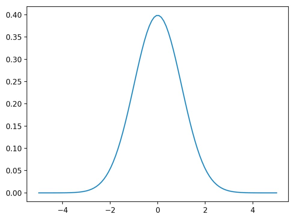
This is the shape we expect so it is likely we have implemented the formula correctly.

Now we need a function that combines everything together. We need the Gaussian PDF value for every $x_i$ , as we talked about above. Then we must multiply all these probabilities together, remembering to also include the $P(c)$ term. Here is a function that achieves this:

python

def PredictClass(model, newData):
  # This function uses the trained model to make a prediction on one new sample of data
  probabilityOfBelongingToEachClassDict = {}

  classes = list(model.keys())

  # Loop through all the possible classes the data could belong to
  for c in classes:
      listOfProbabilitiesToMultiply = []

      # First calculate the probability of the class (proportion of that class in training data)
      listOfProbabilitiesToMultiply.append(CalculateProbabilityOfClassC(c,model))

      # Loop through all attributes of new data and calculate the gaussian pdf value using relevant mean and std.
      for i in range(0, len(newData)):
          listOfProbabilitiesToMultiply.append(GaussianPDF(newData[i], model[c][i][0], model[c][i][1]))

      # Multiply all calculated values together to form probability data belongs to each class
      probabilityOfBelongingToEachClassDict[c] = math.prod(listOfProbabilitiesToMultiply)

  keys = list(probabilityOfBelongingToEachClassDict.keys())
  values = list(probabilityOfBelongingToEachClassDict.values())

  # Choose the class with highest probaiblity associated with it
  predictedClass = keys[values.index(max(values))]

  return predictedClass

We initially calculate the probability of the class $c$ , using the function we wrote earlier, and append it to a list. Then we go through each attribute of the new row of data and calculate $P(x_i|c)$ , and also append these to the same list. Then we multiply that whole list together to produce the number that we will use to estimate the probability that the data belongs to that class. We then repeat this process over all classes. Finally we find the class corresponding to the highest probability calculated (not actual probability however), and choose this as our prediction.

Let's test it! Testing requires producing a train/test split from our full dataset so that we can verify whether the model is able to predict properly or not. Let's import scikit-learn's train_test_split function for this:

python

from sklearn.model_selection import train_test_split
...
if __name__ == '__main__':
  # Load the dataset
  dataFilepath = 'YOUR FILEPATH/iris.data'
  columns = ['sepal-length', 'sepal-width', 'petal-length', 'petal-width', 'class']
  dataset = pd.read_csv(dataFilepath, names=columns)

  # Separate tout the target variable
  X = dataset.drop('class', axis = 1)
  y = dataset['class']

  # Create an 80/20 train/test split
  X_train, X_test, y_train, y_test = train_test_split(X, y, test_size = 0.2, random_state=0)
   
  # Concatenate the training sets
  trainingSet = pd.concat([X_train, y_train], axis = 1)

Here I have created a split where 20% (30 samples) of the data is for testing, and 80% (120 samples) is for training. I concatenate the X_train and y_train sets back together because I implemented my functions assuming that the ‘class’ column was included in the data.

So let’s create the model and train it on the training set:

python

...
model = TrainModel(trainingSet)

We can have a look at it to recall the structure of the model too:

python

...
for x in model.keys():
  print(x)
  print(model[x])

Outputs:

plaintext

Iris-setosa
[[5.02051282051282, 0.36431586004995814, 39], [3.4025641025641025, 0.381470271647932, 39], [1.4615384615384615, 0.144395991735054, 39], [0.2384615384615384, 0.10910011002788757, 39]]
Iris-versicolor
[[5.886486486486487, 0.5207698159467398, 37], [2.7621621621621624, 0.3268973261772905, 37], [4.216216216216216, 0.486206125420481, 37], [1.324324324324324, 0.2046750885962722, 37]]
Iris-virginica
[[6.638636363636363, 0.6310625624426647, 44], [2.9886363636363638, 0.33216408742143666, 44], [5.5659090909090905, 0.5489707840822666, 44], [2.0318181818181817, 0.2567894144676992, 44]]

Let’s test the model on the first sample in the test set. But first we can look at that sample:

python

...
print(X_test.iloc[0])
print(y_test.iloc[0])

Outputs:

plaintext

sepal-length    5.8
sepal-width     2.8
petal-length    5.1
petal-width     2.4

Iris-virginica

So now we can finally test our ‘PredictClass’ function, as follows:

python

...
model = TrainModel(trainingSet)
predictedClass = PredictClass(model, X_test.iloc[0])
print(predictedClass)

This outputs:

plaintext

Iris-virginica

It worked! Out of curiosity, I can modify the ‘PredictClass’ function to instead output the full dictionary of estimated probabilities. That looks like this:

plaintext

{'Iris-setosa': 8.48935365055018e-225,
'Iris-versicolor': 8.701921085911454e-08,
'Iris-virginica': 0.027607489541751216}

The differences are enormous orders of magnitude apart! I believe this is because some of the probabilities we calculate are very small, but then we multiply them all together and, as we know, multiplying very small numbers produces absurdly small numbers! But in any case, we don’t really care about the magnitude of these numbers, we just want to know which one is the largest.

As a quick aside, since these numbers can be incredibly small we risk errors in floating-point precision, such as underflow. This may cause the result of our calculation to be set to 0. To avoid this, some implementations of Naive Bayes methods will instead use log-probabilities, and may also incorporate smoothing functions, such as Laplace smoothing, to avoid results of 0. I won’t be coding these here but I wanted to bring up the concepts.

We’ve done great so far! The last thing to implement is an evaluation function.

4. Calculating our Model’s Accuracy

We can use classification accuracy as a metric here because the classes in our set are balanced. Hence, let’s write a function that predicts the class for each sample in the test set and then checks against ‘y_test’ to see if it was correct.

python

def EvaluateModelAccuracy(model, X_test, y_test):
  # This function uses the trained model to make predictions over a test set, then calculates the accuracy
  predictions = []

  # Loop through all the test data
  for i in range(0,len(X_test)):

      # Make prediction for each new data point
      currentPrediction = PredictClass(model, list(X_test.iloc[i]))

      # Save whether or not the prediction was correct
      if currentPrediction == y_test.iloc[i]:
          predictions.append(1)
      else:
          predictions.append(0)

  # Calculate accuracy
  accuracy = sum(predictions)/len(X_test)
  return accuracy

Now if we call this as follows:

python

...
if __name__ == '__main__':
  # Load the dataset
  dataFilepath = 'YOUR FILEPATH/iris.data'
  columns = ['sepal-length', 'sepal-width', 'petal-length', 'petal-width', 'class']
  dataset = pd.read_csv(dataFilepath, names=columns)

  # Separate out the target variable
  X = dataset.drop('class', axis = 1)
  y = dataset['class']

  # Create a train/test split
  X_train, X_test, y_train, y_test = train_test_split(X, y, test_size = 0.2, random_state=0)

  # Concatenate the target training variable back onto the training set
  trainingSet = pd.concat([X_train, y_train], axis = 1)

  # Train the model on training set
  model = TrainModel(trainingSet)

  # Use the trained model to make predictions on test set, and calculate accuracy of predictions
  modelAccuracy = EvaluateModelAccuracy(model, X_test, y_test)

  print(modelAccuracy)

We get an accuracy rating of:

plaintext

0.9666666666666667

This is a fantastic result! We must of course remember that we’re operating on a very small set (30 test samples) so the scores are not completely reliable but it still shows our model has a great level of skill. Due to the class distribution, if our model had no skill we would expect a baseline accuracy of around 33%. We’re way above that!

And with that, we’re done coding the model and evaluating its performance 🙂

Here is the full code:

python

import pandas as pd
import math
from sklearn.model_selection import train_test_split

def Mean(data):
  return sum(data)/len(data)

def Std(data):
  mu = Mean(data)
  newList = [(x-mu)**2 for x in data]
  return math.sqrt((1/(len(data)-1))*sum(newList))

def GaussianPDF(number, mu, sigma):
  return (1/(sigma*math.sqrt(2*math.pi)))*math.exp(-0.5*((number - mu)/sigma)**2)

def CalculateProbabilityOfClassC(c, model):
  # Function computes the probability of a class c, using counts of how many samples are in each class.
  numberOfSamplesInClassC = model[c][0][2]
  numberOfSamplesInTotal = sum([model[x][0][2] for x in list(model.keys())])
  return numberOfSamplesInClassC/numberOfSamplesInTotal

def SeparateClasses(dataset):
  # Function separates the classes in a dataset, saving the result as a dictionary with classes as the keys.
  separateClassesDict = {}
  dataByClass = dataset.groupby('class')

  for group, data in dataByClass:
      separateClassesDict[group] = data
   
  return separateClassesDict

def CalculateColumnStatsForGivenClass(singleClassDataset):
  # Function calculates the mean, std and sample count for each column, given a single class
  requiredList = []

  # Get all the column names in this class as a list
  cols = list(singleClassDataset.columns)

  # Loop through the list of column names, calculating mean, std, and sample count
  for x in list(cols[0:len(cols)-1]): # -1 because we don't want to include the column for 'class'
      requiredList.append([Mean(singleClassDataset[x]), Std(singleClassDataset[x]), len(singleClassDataset[x])])
  return requiredList

def TrainModel(dataset):
  # Function produces a dictionary representing the Gaussian naive bayes model. 
  result = {}

  # First separate the classes
  dataSeparatedByClassDict = SeparateClasses(dataset)

  # Loop through each class
  for x in list(dataSeparatedByClassDict.keys()):
      # Calculate the mean and std for each attribute, within each class
      result[x] = CalculateColumnStatsForGivenClass(dataSeparatedByClassDict[x])
  return result

def PredictClass(model, newData):
  # This function uses the trained model to make a prediction on one new sample of data
  probabilityOfBelongingToEachClassDict = {}

  classes = list(model.keys())

  # Loop through all the possible classes the data could belong to
  for c in classes:
      listOfProbabilitiesToMultiply = []

      # First calculate the probability of the class (proportion of that class in training data)
      listOfProbabilitiesToMultiply.append(CalculateProbabilityOfClassC(c,model))

      # Loop through all attributes of new data and calculate the gaussian pdf value using relevant mean and std.
      for i in range(0, len(newData)):
          listOfProbabilitiesToMultiply.append(GaussianPDF(newData[i], model[c][i][0], model[c][i][1]))

      # Multiply all calculated values together to form probability data belongs to each class
      probabilityOfBelongingToEachClassDict[c] = math.prod(listOfProbabilitiesToMultiply)

  keys = list(probabilityOfBelongingToEachClassDict.keys())
  values = list(probabilityOfBelongingToEachClassDict.values())

  # Choose the class with highest probaiblity associated with it
  predictedClass = keys[values.index(max(values))]

  return predictedClass

def EvaluateModelAccuracy(model, X_test, y_test):
  # This function uses the trained model to make predictions over a test set, then calculates the accuracy
  predictions = []

  # Loop through all the test data
  for i in range(0,len(X_test)):

      # Make prediction for each new data point
      currentPrediction = PredictClass(model, list(X_test.iloc[i]))

      # Save whether or not the prediction was correct
      if currentPrediction == y_test.iloc[i]:
          predictions.append(1)
      else:
          predictions.append(0)

  # Calculate accuracy
  accuracy = sum(predictions)/len(X_test)
  return accuracy

if __name__ == '__main__':
  # Load the dataset
  dataFilepath = 'YOUR FILEPATH/iris.data'
  columns = ['sepal-length', 'sepal-width', 'petal-length', 'petal-width', 'class']
  dataset = pd.read_csv(dataFilepath, names=columns)

  # Separate out the target variable
  X = dataset.drop('class', axis = 1)
  y = dataset['class']

  # Create a train/test split
  X_train, X_test, y_train, y_test = train_test_split(X, y, test_size = 0.2, random_state=0)

  # Concatenate the target training variable back onto the training set
  trainingSet = pd.concat([X_train, y_train], axis = 1)

  # Train the model on training set
  model = TrainModel(trainingSet)

  # Use the trained model to make predictions on test set, and calculate accuracy of predictions
  modelAccuracy = EvaluateModelAccuracy(model, X_test, y_test)

  print(modelAccuracy)

Extension Tasks

We have successfully coded all the basic functions of a Gaussian Naive Bayes classifier, however there are a variety of extensions you could choose to implement at this point.

Try different probability density functions. We choose to use a Gaussian density function but other densities can be used too. Try implementing Bernoulli or Multinomial probability density functions.
Try a different dataset. We have applied our classifier to perhaps the simplest dataset that exists. Maybe you could try and implement it on a larger set and analyse the performance that our model achieves when compared to scikit-learn’s implementation, say.
Handle categorical variables. A problem you may encounter when implementing the model on another dataset is categorical variables – we cannot calculate their mean and standard deviation. Instead, the solution is to compute the ratio of category values for each class and use this instead.
Laplace smoothing. If any $P(x_i|c)$ ends up being calculated as 0, we will get a probability value of 0 for that piece of data belonging to that class. Of course this should never be the case (there’s always a chance it belongs to each class) so a technique to fix it is Laplace smoothing. Try implementing it (or simply researching it)!
Log probabilities. You saw earlier that one of our class probability values was of the order of 10e-225! This is worrying small and threatens to cause issues with floating point precision. One way of helping this is to take the log of the probability values.

Conclusion

We have covered the theory behind the Naive Bayes methods and even implemented one by hand in Python! We used a very simple dataset as a way to prove our implementation works, and we achieved 96% classification accuracy!

If you’ve not already started, I encourage you to try implementing this model yourself in Python! Or if you’d rather study and play around with my code, you can copy it from above or find it at this GitHub link.

Thanks for reading, hope you enjoyed!